在线工具推荐：三维数字孪生场景工具 - GLTF/GLB在线编辑器 - Three.js AI自动纹理化开发 - YOLO 虚幻合成数据生成器 - 3D模型在线转换 -  3D模型预览图生成服务

ChatGPT 已经成为一把可用于多种应用的瑞士军刀，并且有大量的空间将 ChatGPT 集成到数据科学工作流程中。

如果您曾经在真实数据集上训练过机器学习模型，您就会知道数据清理和预处理的步骤对于构建可靠的机器学习模型非常重要。在本指南中，我们将了解如何使用 ChatGPT 在示例数据集上执行这些任务。

我们将使用 UCI 机器学习存储库中的银行营销数据集，并提示 ChatGPT 执行以下操作：

• 获取并加载数据集
• 检查缺失值
• 对分类变量进行编码

您可以通过登录您的 OpenAI 帐户并开始新的 ChatGPT 会话来跟进。如果你愿意，你也可以在谷歌Colab中编码。

获取和加载数据集

数据集有几个不同版本。我们将使用银行满.csv。

提示：今天我们将对真实数据集进行数据清理和预处理。编写代码以执行以下操作：1. 从 UCI 机器学习存储库中提取银行营销数据集。使用请求或 urllib 等库。2. 下载 zip 文件，解压缩内容，并将银行已满.csv文件读取到 pandas 数据帧中（称为数据）。

在数据集中获取和读取的代码如下：

import pandas as pd
import urllib
import zipfile

# URL of the dataset
url = "https://archive.ics.uci.edu/ml/machine-learning-databases/00222/bank.zip"

# Fetch and extract the dataset
urllib.request.urlretrieve(url, "bank.zip")

with zipfile.ZipFile("bank.zip", "r") as zip_ref:
    zip_ref.extractall()

# Load the dataset into a pandas DataFrame
data = pd.read_csv("bank-full.csv", delimiter=";",skipinitialspace=True)

获取数据集的基本信息

让我们更好地理解数据集。

# Display the first few rows of the dataset
print(data.head())

这输出：

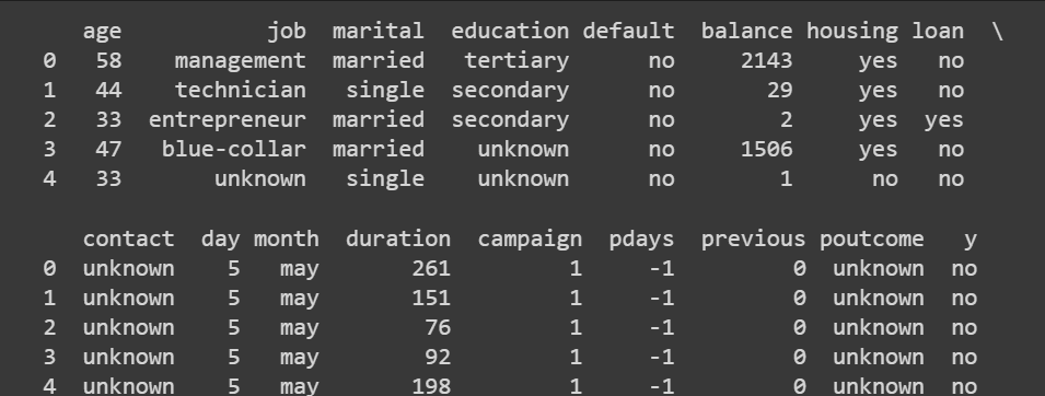
截断的输出 data.head（）

提示：使用 pandas 获取数据帧的维度、列的描述性统计信息以及各种列的数据类型。

这一步并不需要提示 ChatGPT，因为 pandas 方法非常简单。

# Get the dimensions of the dataset (rows, columns)
print(data.shape)

Output >>> (45211, 17)

我们有超过 45000 条记录和 16 个特征（因为 17 个也包括输出标签）。

# Get statistical summary of numerical columns
print(data.describe())

数据.describe（） 的截断输出

获取各个列的数据类型的概述也很有帮助。当我们对分类变量进行编码时，我们将仔细研究它们。

# Check data types of each column
print(data.dtypes)

Output >>>

age           int64
job          object
marital      object
education    object
default      object
balance       int64
housing      object
loan         object
contact      object
day           int64
month        object
duration      int64
campaign      int64
pdays         int64
previous      int64
poutcome     object
y            object
dtype: object

到目前为止，我们已经了解了银行营销数据集。输出标签表示客户是否会订阅定期存款。该数据集包含多个要素，例如年龄、月份、教育程度、婚姻状况、先前广告系列的结果等。

检查缺失值

提示：我想知道每列中缺失值的数量。请给我代码来做这件事。使用熊猫。

# Check for missing values in each column
missing_values = data.isnull().sum()
print(missing_values)

下面是输出：

Output >>>

age          0
job          0
marital      0
education    0
default      0
balance      0
housing      0
loan         0
contact      0
day          0
month        0
duration     0
campaign     0
pdays        0
previous     0
poutcome     0
y            0
dtype: int64

此版本的银行营销数据集（包含超过 45000 条记录）没有任何缺失值。但实际上，大多数真实世界的数据集都有缺失值。您应该使用合适的插补技术来处理缺失值。

作为可选的练习，您可以在此处添加一个步骤，提示 ChatGPT 从列的子集中删除一小部分值，以便您可以练习如何处理缺失值。

编码分类变量

下一步是对数据集中的分类变量进行编码。我们将首先获取所有分类列的列表。

提示：提供代码以获取此数据集中所有分类列的列表。

# Count the number of categorical variables
categorical_columns = data.select_dtypes(include=['object']).columns
print(categorical_columns)
num_categorical_variables = len(categorical_columns)

# Display the count
print("Number of categorical variables:", num_categorical_variables)

分类列列表还包括输出标签 y。但是，让我们先关注其他分类变量。

Output >>>
Index(['job', 'marital', 'education', 'default', 'housing', 'loan', 'contact',
       'month', 'poutcome', 'y'],
      dtype='object')
Number of categorical variables: 10

仔细查看分类变量的值

接下来，让我们看看每个分类变量采用的值。

提示：我想了解每个分类变量采用的各种值。给熊猫代码来做到这一点。

# Get the different values and their counts for each categorical column
categorical_columns = ['job', 'marital', 'education', 'default', 'housing', 'loan', 'contact', 'month', 'poutcome']
for column in categorical_columns:
    value_counts = data[column].value_counts()
    print(f"Column: {column}")
    print(value_counts,"\n")

输出很难解析：

Output >>>

Column: job
blue-collar      9732
management       9458
technician       7597
admin.           5171
services         4154
retired          2264
self-employed    1579
entrepreneur     1487
unemployed       1303
housemaid        1240
student           938
unknown           288
Name: job, dtype: int64 

...
...
...
Column: poutcome
unknown    36959
failure     4901
other       1840
success     1511
Name: poutcome, dtype: int64 

可视化分类变量的值

让我们提示 ChatGPT 创建一个可视化，以便更容易理解分类变量采用的值。

提示：我想要一个显示每个分类变量取值的图。排除输出标签 y。包括所有其他分类变量。

我们开始吧！

import matplotlib.pyplot as plt

# Get the different values and their counts for each categorical column
categorical_columns = ['job', 'marital', 'education', 'default', 'housing', 'loan', 'contact', 'month', 'poutcome']

# Set up the subplot grid
fig, axes = plt.subplots(3, 3, figsize=(10,8))

# Iterate over each categorical column and plot the value counts
for i, column in enumerate(categorical_columns):
    row = i // 3
    col = i % 3
    value_counts = data[column].value_counts()
    ax = axes[row, col]
    value_counts.plot(kind='bar', ax=ax)
    ax.set_xlabel(column)
    ax.set_ylabel('Count')
    ax.set_title(f'{column.title()} Value Counts')

# Adjust spacing between subplots
plt.tight_layout()

# Show the plot
plt.show()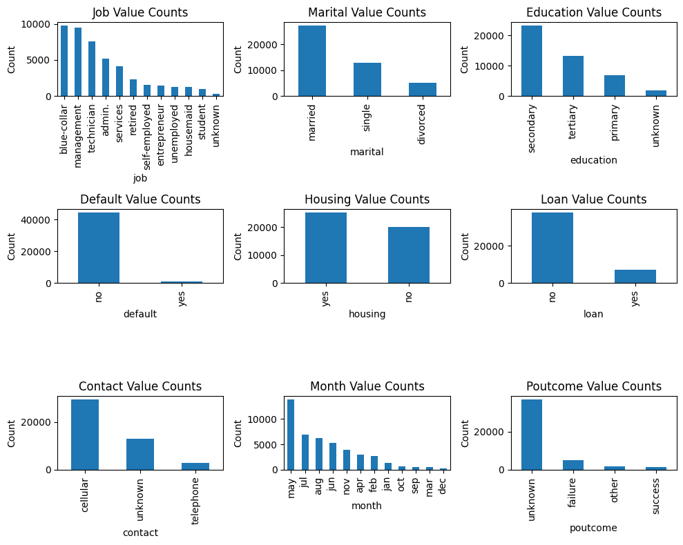

分类变量的值

独热编码

对于分类列的子集，我们可以使用独热编码。

提示：给 pandas 代码以对列列表执行独热编码。

我们使用从熊猫到独热编码以下列：get_dummies

# Select the categorical columns (excluding education and poutcome)
categorical_columns = ['job', 'marital', 'default', 'housing', 'loan', 'contact']

# Perform one-hot encoding
encoded_data = pd.get_dummies(data, columns=categorical_columns)

提示：我想打印出新添加列的前几行。编写代码以执行相同的操作。

# Select the newly added columns
new_columns = encoded_data.columns.difference(data.columns)

# Print the head of the newly added columns
print(encoded_data[new_columns].head())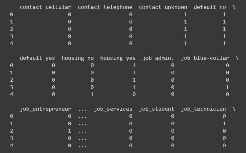

截断的输出 encoded_data['new_colums'].head（）

定义自定义映射

对于“education”和“poutcome”（先前结果）等变量的列，而不是独热编码，最好使用自定义映射在值之间进行一定程度的比较。

此外，当我们使用独热编码来编码一个分类变量时，该变量采用 k 个不同的值 k 个新列。对于像“月”这样的分类列，如果不添加太多信息，这将是多余的。

因此，对于这两种情况，我们将定义一个自定义映射，然后转换值。我们可以提示 ChatGPT 获取一个通用代码片段，然后我们可以修改该代码片段以定义特定列的映射。

提示：我想做一个自定义映射来编码一些分类变量。首先给我一个通用代码片段，该代码片段定义了从分类列中的唯一值到一组不同输出值的自定义映射。然后，我们应该使用此映射来转换列中的值。

# Define the custom mapping dictionary
custom_mapping = {
    'category1': 'value1',
    'category2': 'value2',
    'category3': 'value3',
    # Add more categories and corresponding values as needed
}

# Specify the categorical column
categorical_column = 'column_name'  # Replace 'column_name' with the actual column name

# Perform the mapping using the custom mapping dictionary
data[categorical_column] = data[categorical_column].map(custom_mapping)

对于“月”列，让我们像这样转换月份字符串：

# Define the mapping dictionary for months
month_mapping = {
    'jan': 1,
    'feb': 2,
    'mar': 3,
    'apr': 4,
    'may': 5,
    'jun': 6,
    'jul': 7,
    'aug': 8,
    'sep': 9,
    'oct': 10,
    'nov': 11,
    'dec': 12
}

# Map the values in the month column
encoded_data['month'] = encoded_data['month'].map(month_mapping)

让我们将“结果”和“教育”列映射到数值，如下所示：

# Define the custom mapping for poutcome and education
poutcome_mapping = {
    'unknown': 0,
    'failure': 1,
    'other': 2,
    'success': 3
}

education_mapping = {
    'unknown': 0,
    'primary': 1,
    'secondary': 2,
    'tertiary': 3
}

# Perform ordinal encoding using pandas map
encoded_data['poutcome'] = encoded_data['poutcome'].map(poutcome_mapping)
encoded_data['education'] = encoded_data['education'].map(education_mapping)


# Select the newly added columns
new_columns = ['month','poutcome', 'education']

# Print the head of the newly added columns
print(encoded_data[new_columns].head(10))

对输出标签进行编码

我们还将输出标签“是”和“否”分别映射到 1 和 0。

encoded_data['y'] = encoded_data['y'].replace({'no': 0, 'yes': 1})
print(encoded_data['y'])

Output >>>

0        0
1        0
2        0
3        0
4        0
        ..
45206    1
45207    1
45208    1
45209    0
45210    0
Name: y, Length: 45211, dtype: int64

回想一下，我们对“住房”、“默认”和“贷款”列使用了独热编码。由于这些列还采用“是”和“否”值，因此您还可以将“是”和“否”分别映射到 1 和 0。

可视化类标签的分布

检查类标签的分布也很有帮助，这样我们就可以在需要时在构建模型时考虑类不平衡。

提示：我想了解类标签的分布。请给我代码以生成合适的图。

以下是在Seaborn中生成计数图的代码：

import seaborn as sns
import matplotlib.pyplot as plt

# Plot the distribution of output labels
sns.countplot(data=data, x='y')
plt.xlabel('Output Label')
plt.ylabel('Count')
plt.title('Output Label Distribution')
plt.show()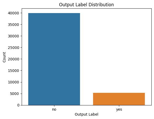

类标签的分发

我们看到存在阶级失衡。因此，如果要构建模型，则应确保使用适当的重采样方法解决类不平衡问题。

通用数据清理和预处理管道

尽管数据清理和预处理需要开发人员的努力，但让我们尝试获取一个通用的步骤序列，该步骤序列对于简单的数据集来说相当有效。

提示：您能否根据我们到目前为止所做的工作给我一个通用的数据清理和预处理管道。获取数据集的基本信息，检查和处理缺失值，标识分类列，并对分类列进行编码。只使用熊猫。

这是：

import pandas as pd

# Load the dataset into a DataFrame
data = pd.read_csv('data.csv')

# Step 1: Basic Info
print(data.info())

# Step 2: Missing Values
missing_values = data.isnull().sum()
print(missing_values)

# Step 3: Handle Missing Values
# Identify columns with missing values
columns_with_missing_values = missing_values[missing_values > 0].index

# Impute missing values using fillna() or other suitable method
data[columns_with_missing_values] = data[columns_with_missing_values].fillna(data[columns_with_missing_values].mean())

# Step 4: Get Categorical Columns
categorical_columns = data.select_dtypes(include=['object']).columns

# Step 5: Encode Categorical Columns
# Perform ordinal encoding or one-hot encoding using pandas' get_dummies() function
encoded_data = pd.get_dummies(data, columns=categorical_columns)

# Print the encoded data
print(encoded_data.head())

总结

可以看出，与 ChatGPT 协同作用的数据科学专业知识可以帮助使数据清理和预处理更简单、更快捷。现在，您已经准备好了预处理的数据集，您可以通过在此银行营销数据集上构建一个简单的预测模型来进一步实现这一点。

由3D建模学习工作室 整理翻译，转载请注明出处！