在 PyTorch 中构建逻辑回归分类器
逻辑回归的公式是将 sigmoid 函数应用于线性函数的输出。本文讨论如何构建逻辑回归分类器。虽然之前您一直在处理单变量数据集,但在这里我们将使用流行的 MNIST 数据集来训练和测试我们的模型
推荐:将NSDT场景编辑器加入你的3D工具链
3D工具集:NSDT简石数字孪生
在 PyTorch 中构建逻辑回归分类器
逻辑回归是一种预测事件概率的回归。它用于分类问题,在机器学习、人工智能和数据挖掘领域有许多应用。
逻辑回归的公式是将 sigmoid 函数应用于线性函数的输出。本文讨论如何构建逻辑回归分类器。虽然之前您一直在处理单变量数据集,但在这里我们将使用流行的 MNIST 数据集来训练和测试我们的模型。阅读本文后,您将了解:
- 如何在 PyTorch 中使用逻辑回归以及如何将其应用于现实世界的问题。
- 如何加载和分析火炬视觉数据集。
- 如何在图像数据集上构建和训练逻辑回归分类器。

在 PyTorch 中构建逻辑回归分类器。
图片来自猫女变种人。保留部分权利。
概述
本教程分为四个部分;他们是
- MNIST 数据集
- 将数据集加载到数据加载器
- 构建模型
nn.Module - 训练分类器
MNIST 数据集
您将使用 MNIST 数据集训练和测试逻辑回归模型。此数据集包含 6000 张用于训练的图像和 10000 张用于测试样本外性能的图像。
MNIST数据集非常受欢迎,以至于它是PyTorch的一部分。下面介绍如何在 PyTorch 中加载 MNIST 数据集的训练和测试样本。
1 2 3 4 5 6 7 8 9 10 11 12 13 | import torch import torchvision.transforms as transforms from torchvision import datasets # loading training data train_dataset = datasets.MNIST(root='./data', train=True, transform=transforms.ToTensor(), download=True) #loading test data test_dataset = datasets.MNIST(root='./data', train=False, transform=transforms.ToTensor()) |
数据集将被下载并提取到目录,如下所示。
1 2 3 4 5 6 7 8 9 10 11 12 13 14 15 16 17 18 19 | Downloading http://yann.lecun.com/exdb/mnist/train-images-idx3-ubyte.gz Downloading http://yann.lecun.com/exdb/mnist/train-images-idx3-ubyte.gz to ./data/MNIST/raw/train-images-idx3-ubyte.gz 0%| | 0/9912422 [00:00<?, ?it/s] Extracting ./data/MNIST/raw/train-images-idx3-ubyte.gz to ./data/MNIST/raw Downloading http://yann.lecun.com/exdb/mnist/train-labels-idx1-ubyte.gz Downloading http://yann.lecun.com/exdb/mnist/train-labels-idx1-ubyte.gz to ./data/MNIST/raw/train-labels-idx1-ubyte.gz 0%| | 0/28881 [00:00<?, ?it/s] Extracting ./data/MNIST/raw/train-labels-idx1-ubyte.gz to ./data/MNIST/raw Downloading http://yann.lecun.com/exdb/mnist/t10k-images-idx3-ubyte.gz Downloading http://yann.lecun.com/exdb/mnist/t10k-images-idx3-ubyte.gz to ./data/MNIST/raw/t10k-images-idx3-ubyte.gz 0%| | 0/1648877 [00:00<?, ?it/s] Extracting ./data/MNIST/raw/t10k-images-idx3-ubyte.gz to ./data/MNIST/raw Downloading http://yann.lecun.com/exdb/mnist/t10k-labels-idx1-ubyte.gz Downloading http://yann.lecun.com/exdb/mnist/t10k-labels-idx1-ubyte.gz to ./data/MNIST/raw/t10k-labels-idx1-ubyte.gz 0%| | 0/4542 [00:00<?, ?it/s] Extracting ./data/MNIST/raw/t10k-labels-idx1-ubyte.gz to ./data/MNIST/raw |
让我们验证数据集中的训练和测试样本数。
1 2 | print("number of training samples: " + str(len(train_dataset)) + "\n" + "number of testing samples: " + str(len(test_dataset))) |
它打印
1 2 | number of training samples: 60000 number of testing samples: 10000 |
数据集中的每个样本都是一对图像和标签。若要检查训练数据中第一个元素的数据类型和大小,可以使用 和 方法。type()size()
1 2 | print("datatype of the 1st training sample: ", train_dataset[0][0].type()) print("size of the 1st training sample: ", train_dataset[0][0].size()) |
这打印
1 2 | datatype of the 1st training sample: torch.FloatTensor size of the 1st training sample: torch.Size([1, 28, 28]) |
可以使用列表索引从数据集访问示例。数据集中的第一个样本是一个,它是一个 $28\times 28$ 像素的灰度图像(即一个通道),因此大小 .FloatTensor[1, 28, 28]
现在,让我们检查训练集中前两个样本的标签。
1 2 3 | # check the label of first two training sample print("label of the first taining sample: ", train_dataset[0][1]) print("label of the second taining sample: ", train_dataset[1][1]) |
这显示了
1 2 | label of the first taining sample: 5 label of the second taining sample: 0 |
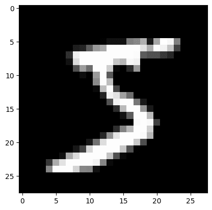
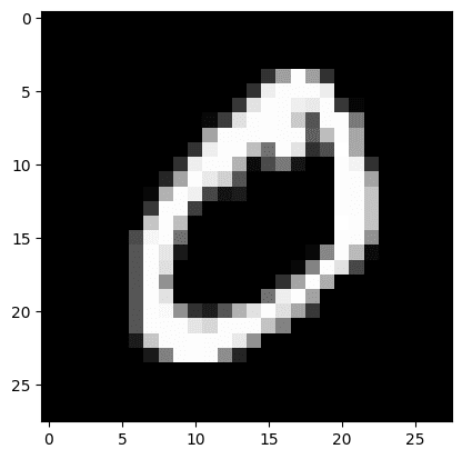
从上面可以看出,训练集中的前两个图像代表“5”和“0”。让我们展示这两个图像来确认。
1 2 3 4 5 6 | img_5 = train_dataset[0][0].numpy().reshape(28, 28) plt.imshow(img_5, cmap='gray') plt.show() img_0 = train_dataset[1][0].numpy().reshape(28, 28) plt.imshow(img_0, cmap='gray') plt.show() |
您应该看到以下两位数字:
将数据集加载到数据加载器
通常,您不会直接在训练中使用数据集,而是通过类使用数据集。这允许您批量读取数据,而不是样本。DataLoader
在下文中,数据被加载到批大小为 32 的 中。DataLoader
1 2 3 4 5 6 7 | ... from torch.utils.data import DataLoader # load train and test data samples into dataloader batach_size = 32 train_loader = DataLoader(dataset=train_dataset, batch_size=batach_size, shuffle=True) test_loader = DataLoader(dataset=test_dataset, batch_size=batach_size, shuffle=False) |
Want to Get Started With Building Transformer Models with Attention?
Take my free 12-day email crash course now (with sample code).
Click to sign-up and also get a free PDF Ebook version of the course.
Download Your FREE Mini-Course
Build the Model with nn.Module
Let’s build the model class with for our logistic regression model. This class is similar to that in the previous posts but the numbers of input and output are configurable.nn.Module
1 2 3 4 5 6 7 8 9 10 | # build custom module for logistic regression class LogisticRegression(torch.nn.Module): # build the constructor def __init__(self, n_inputs, n_outputs): super(LogisticRegression, self).__init__() self.linear = torch.nn.Linear(n_inputs, n_outputs) # make predictions def forward(self, x): y_pred = torch.sigmoid(self.linear(x)) return y_pred |
This model will take a 28×28-pixel image of handwritten digits as input and classify them into one of the 10 output classes of digits 0 to 9. So, here is how you can instantiate the model.
1 2 3 4 | # instantiate the model n_inputs = 28*28 # makes a 1D vector of 784 n_outputs = 10 log_regr = LogisticRegression(n_inputs, n_outputs) |
Training the Classifier
You will train this model with stochastic gradient descent as the optimizer with learning rate 0.001 and cross-entropy as the loss metric.
Then, the model is trained for 50 epochs. Note that you have use method to flatten the image matrices into rows to fit the same of the logistic regression model input.view()
1 2 3 4 5 6 7 8 9 10 11 12 13 14 15 16 17 18 19 20 21 22 23 24 25 26 27 | ... # defining the optimizer optimizer = torch.optim.SGD(log_regr.parameters(), lr=0.001) # defining Cross-Entropy loss criterion = torch.nn.CrossEntropyLoss() epochs = 50 Loss = [] acc = [] for epoch in range(epochs): for i, (images, labels) in enumerate(train_loader): optimizer.zero_grad() outputs = log_regr(images.view(-1, 28*28)) loss = criterion(outputs, labels) # Loss.append(loss.item()) loss.backward() optimizer.step() Loss.append(loss.item()) correct = 0 for images, labels in test_loader: outputs = log_regr(images.view(-1, 28*28)) _, predicted = torch.max(outputs.data, 1) correct += (predicted == labels).sum() accuracy = 100 * (correct.item()) / len(test_dataset) acc.append(accuracy) print('Epoch: {}. Loss: {}. Accuracy: {}'.format(epoch, loss.item(), accuracy)) |
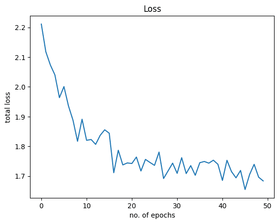
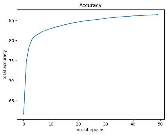
在训练期间,应会看到如下所示的进度:
1 2 3 4 5 6 7 8 9 10 11 12 | Epoch: 0. Loss: 2.211054563522339. Accuracy: 61.63 Epoch: 1. Loss: 2.1178536415100098. Accuracy: 74.81 Epoch: 2. Loss: 2.0735440254211426. Accuracy: 78.47 Epoch: 3. Loss: 2.040225028991699. Accuracy: 80.17 Epoch: 4. Loss: 1.9637292623519897. Accuracy: 81.05 Epoch: 5. Loss: 2.000900983810425. Accuracy: 81.44 ... Epoch: 45. Loss: 1.6549798250198364. Accuracy: 86.3 Epoch: 46. Loss: 1.7053509950637817. Accuracy: 86.31 Epoch: 47. Loss: 1.7396119832992554. Accuracy: 86.36 Epoch: 48. Loss: 1.6963073015213013. Accuracy: 86.37 Epoch: 49. Loss: 1.6838685274124146. Accuracy: 86.46 |
通过仅对模型进行 86 个 epoch 的训练,您就实现了大约 50% 的准确率。如果模型训练时间更长,则可以进一步提高准确性。
让我们可视化损失和准确性的图形。以下是损失:
1 2 3 4 5 | plt.plot(Loss) plt.xlabel("no. of epochs") plt.ylabel("total loss") plt.title("Loss") plt.show() |
这是为了准确:
1 2 3 4 5 | plt.plot(acc) plt.xlabel("no. of epochs") plt.ylabel("total accuracy") plt.title("Accuracy") plt.show() |
将所有内容放在一起,以下是完整的代码:
1 2 3 4 5 6 7 8 9 10 11 12 13 14 15 16 17 18 19 20 21 22 23 24 25 26 27 28 29 30 31 32 33 34 35 36 37 38 39 40 41 42 43 44 45 46 47 48 49 50 51 52 53 54 55 56 57 58 59 60 61 62 63 64 65 66 67 68 69 70 71 72 73 74 75 76 77 78 79 80 81 82 83 84 85 86 87 88 89 90 | import torch import torchvision.transforms as transforms from torchvision import datasets from torch.utils.data import DataLoader import matplotlib.pyplot as plt # loading training data train_dataset = datasets.MNIST(root='./data', train=True, transform=transforms.ToTensor(), download=True) # loading test data test_dataset = datasets.MNIST(root='./data', train=False, transform=transforms.ToTensor()) print("number of training samples: " + str(len(train_dataset)) + "\n" + "number of testing samples: " + str(len(test_dataset))) print("datatype of the 1st training sample: ", train_dataset[0][0].type()) print("size of the 1st training sample: ", train_dataset[0][0].size()) # check the label of first two training sample print("label of the first taining sample: ", train_dataset[0][1]) print("label of the second taining sample: ", train_dataset[1][1]) img_5 = train_dataset[0][0].numpy().reshape(28, 28) plt.imshow(img_5, cmap='gray') plt.show() img_0 = train_dataset[1][0].numpy().reshape(28, 28) plt.imshow(img_0, cmap='gray') plt.show() # load train and test data samples into dataloader batach_size = 32 train_loader = DataLoader(dataset=train_dataset, batch_size=batach_size, shuffle=True) test_loader = DataLoader(dataset=test_dataset, batch_size=batach_size, shuffle=False) # build custom module for logistic regression class LogisticRegression(torch.nn.Module): # build the constructor def __init__(self, n_inputs, n_outputs): super().__init__() self.linear = torch.nn.Linear(n_inputs, n_outputs) # make predictions def forward(self, x): y_pred = torch.sigmoid(self.linear(x)) return y_pred # instantiate the model n_inputs = 28*28 # makes a 1D vector of 784 n_outputs = 10 log_regr = LogisticRegression(n_inputs, n_outputs) # defining the optimizer optimizer = torch.optim.SGD(log_regr.parameters(), lr=0.001) # defining Cross-Entropy loss criterion = torch.nn.CrossEntropyLoss() epochs = 50 Loss = [] acc = [] for epoch in range(epochs): for i, (images, labels) in enumerate(train_loader): optimizer.zero_grad() outputs = log_regr(images.view(-1, 28*28)) loss = criterion(outputs, labels) # Loss.append(loss.item()) loss.backward() optimizer.step() Loss.append(loss.item()) correct = 0 for images, labels in test_loader: outputs = log_regr(images.view(-1, 28*28)) _, predicted = torch.max(outputs.data, 1) correct += (predicted == labels).sum() accuracy = 100 * (correct.item()) / len(test_dataset) acc.append(accuracy) print('Epoch: {}. Loss: {}. Accuracy: {}'.format(epoch, loss.item(), accuracy)) plt.plot(Loss) plt.xlabel("no. of epochs") plt.ylabel("total loss") plt.title("Loss") plt.show() plt.plot(acc) plt.xlabel("no. of epochs") plt.ylabel("total accuracy") plt.title("Accuracy") plt.show() |
总结
在本教程中,您学习了如何在 PyTorch 中构建多类逻辑回归分类器。特别是,你学到了。
- 如何在 PyTorch 中使用逻辑回归以及如何将其应用于现实世界的问题。
- 如何加载和分析火炬视觉数据集。
- 如何在图像数据集上构建和训练逻辑回归分类器。
由3D建模学习工作室 翻译整理,转载请注明出处!