PyTorch创建图像数据Softmax 分类器
Softmax分类器是监督学习中的一种分类器。它是深度学习网络中的重要构建块,也是深度学习从业者中最受欢迎的选择。 Softmax分类器适用于多类分类,它输出每个类的概率。

推荐:将NSDT场景编辑器加入你的3D工具链
本教程将教您如何为图像数据构建softmax分类器。您将学习如何准备数据集,然后学习如何使用 PyTorch 实现 softmax 分类器。特别是,您将学习:
- 关于 Fashion-MNIST 数据集。
- 如何在 PyTorch 中对图像使用 Softmax 分类器。
- 如何在 PyTorch 中构建和训练多类图像分类器。
- 如何在模型训练后绘制结果。
用我的书《Deep Learning with PyTorch》开始你的项目。它提供了带有工作代码的自学教程。
让我们开始吧。

概述
本教程分为三个部分,他们是:
- 准备数据集
- 构建模型
- 训练模型
准备数据集
您将在此处使用的数据集是Fashion-MNIST。它是一个经过预处理且组织良好的数据集,由 70,000 张图像组成,其中 60,000 张图像用于训练数据,10,000 张图像用于测试数据。
数据集中的每个示例都是一个28×28像素灰度图像,总像素数为 784。数据集有 10 个类,每个图像都标记为时尚项目,该项目与 0 到 9 的整数标签相关联。
可以从 加载此数据集。为了使训练更快,我们将数据集限制为 4000 个样本:torchvision
1 2 3 4 | from torchvision import datasets train_data = datasets.FashionMNIST('data', train=True, download=True) train_data = list(train_data)[:4000] |
在你第一次获取fashion-MNIST数据集时,你会看到PyTorch从互联网下载它并保存到一个名为的本地目录中:data
1 2 3 4 5 6 7 8 9 10 11 12 13 14 15 16 17 18 | Downloading http://fashion-mnist.s3-website.eu-central-1.amazonaws.com/train-images-idx3-ubyte.gz Downloading http://fashion-mnist.s3-website.eu-central-1.amazonaws.com/train-images-idx3-ubyte.gz to data/FashionMNIST/raw/train-images-idx3-ubyte.gz 0%| | 0/26421880 [00:00<?, ?it/s] Extracting data/FashionMNIST/raw/train-images-idx3-ubyte.gz to data/FashionMNIST/raw Downloading http://fashion-mnist.s3-website.eu-central-1.amazonaws.com/train-labels-idx1-ubyte.gz Downloading http://fashion-mnist.s3-website.eu-central-1.amazonaws.com/train-labels-idx1-ubyte.gz to data/FashionMNIST/raw/train-labels-idx1-ubyte.gz 0%| | 0/29515 [00:00<?, ?it/s] Extracting data/FashionMNIST/raw/train-labels-idx1-ubyte.gz to data/FashionMNIST/raw Downloading http://fashion-mnist.s3-website.eu-central-1.amazonaws.com/t10k-images-idx3-ubyte.gz Downloading http://fashion-mnist.s3-website.eu-central-1.amazonaws.com/t10k-images-idx3-ubyte.gz to data/FashionMNIST/raw/t10k-images-idx3-ubyte.gz 0%| | 0/4422102 [00:00<?, ?it/s] Extracting data/FashionMNIST/raw/t10k-images-idx3-ubyte.gz to data/FashionMNIST/raw Downloading http://fashion-mnist.s3-website.eu-central-1.amazonaws.com/t10k-labels-idx1-ubyte.gz Downloading http://fashion-mnist.s3-website.eu-central-1.amazonaws.com/t10k-labels-idx1-ubyte.gz to data/FashionMNIST/raw/t10k-labels-idx1-ubyte.gz 0%| | 0/5148 [00:00<?, ?it/s] Extracting data/FashionMNIST/raw/t10k-labels-idx1-ubyte.gz to data/FashionMNIST/raw |
上面的数据集是一个元组列表,每个元组都是一个图像(以 Python 映像库对象的形式)和一个整数标签。train_data
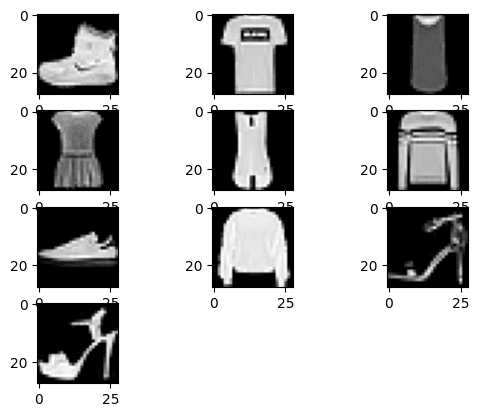
让我们使用 matplotlib 绘制数据集中的前 10 张图像。
1 2 3 4 5 6 7 8 | import matplotlib.pyplot as plt # plot the first 10 images in the training data for i, (img, label) in enumerate(train_data[:10]): plt.subplot(4, 3, i+1) plt.imshow(img, cmap="gray") plt.show() |
您应该看到如下所示的图像:
PyTorch 需要 PyTorch 张量中的数据集。因此,您将使用 PyTorch 转换中的方法通过应用转换来转换此数据。这种转换可以在Torchvision的数据集API中透明地完成:ToTensor()
1 2 3 4 5 | from torchvision import datasets, transforms # download and apply the transform train_data = datasets.FashionMNIST('data', train=True, download=True, transform=transforms.ToTensor()) train_data = list(train_data)[:4000] |
在继续模型之前,我们还将数据拆分为训练集和验证集,以便前 3500 张图像是训练集,其余图像用于验证。通常我们想在拆分之前打乱数据,但我们可以跳过此步骤以使代码简洁。
1 2 | # splitting the dataset into train and validation sets train_data, val_data = train_data[:3500], train_data[3500:] |
想开始使用 PyTorch 进行深度学习吗?
立即参加我的免费电子邮件速成课程(带有示例代码)。
单击以注册并获得该课程的免费PDF电子书版本。
下载您的免费迷你课程
构建模型
为了构建用于图像分类的自定义softmax模块,我们将使用PyTorch库中的模块。为了简单起见,我们构建了一个仅包含一层的模型。nn.Module
1 2 3 4 5 6 7 8 9 10 11 | import torch # build custom softmax module class Softmax(torch.nn.Module): def __init__(self, n_inputs, n_outputs): super().__init__() self.linear = torch.nn.Linear(n_inputs, n_outputs) def forward(self, x): pred = self.linear(x) return pred |
现在,让我们实例化我们的模型对象。它采用一维向量作为输入,并预测 10 个不同的类。我们还检查一下参数是如何初始化的。
1 2 3 | # call Softmax Classifier model_softmax = Softmax(784, 10) print(model_softmax.state_dict()) |
您应该看到模型的权重是随机初始化的,但它的形状应如下所示:
1 2 3 4 5 6 7 8 9 10 11 | OrderedDict([('linear.weight', tensor([[-0.0344, 0.0334, -0.0278, ..., -0.0232, 0.0198, -0.0123], [-0.0274, -0.0048, -0.0337, ..., -0.0340, 0.0274, -0.0091], [ 0.0078, -0.0057, 0.0178, ..., -0.0013, 0.0322, -0.0219], ..., [ 0.0158, -0.0139, -0.0220, ..., -0.0054, 0.0284, -0.0058], [-0.0142, -0.0268, 0.0172, ..., 0.0099, -0.0145, -0.0154], [-0.0172, -0.0224, 0.0016, ..., 0.0107, 0.0147, 0.0252]])), ('linear.bias', tensor([-0.0156, 0.0061, 0.0285, 0.0065, 0.0122, -0.0184, -0.0197, 0.0128, 0.0251, 0.0256]))]) |
训练模型
您将使用随机梯度下降法进行模型训练以及交叉熵损失。让我们将学习率固定为 0.01。为了帮助训练,我们还将数据加载到训练集和验证集的数据加载器中,并将批大小设置为 16。
1 2 3 4 5 6 7 8 9 | class Softmax(torch.nn.Module): "custom softmax module" def __init__(self, n_inputs, n_outputs): super().__init__() self.linear = torch.nn.Linear(n_inputs, n_outputs) def forward(self, x): pred = self.linear(x) return pred |
现在,让我们把所有东西放在一起,训练我们的模型 200 个 epoch。
1 2 3 4 5 6 7 8 9 10 11 12 13 14 15 16 17 18 19 20 21 | epochs = 200 Loss = [] acc = [] for epoch in range(epochs): for i, (images, labels) in enumerate(train_loader): optimizer.zero_grad() outputs = model_softmax(images.view(-1, 28*28)) loss = criterion(outputs, labels) # Loss.append(loss.item()) loss.backward() optimizer.step() Loss.append(loss.item()) correct = 0 for images, labels in val_loader: outputs = model_softmax(images.view(-1, 28*28)) _, predicted = torch.max(outputs.data, 1) correct += (predicted == labels).sum() accuracy = 100 * (correct.item()) / len(val_data) acc.append(accuracy) if epoch % 10 == 0: print('Epoch: {}. Loss: {}. Accuracy: {}'.format(epoch, loss.item(), accuracy)) |
You should see the progress printed once every 10 epochs:
1 2 3 4 5 6 7 8 9 10 11 12 13 14 15 16 17 18 19 20 | Epoch: 0. Loss: 1.0223602056503296. Accuracy: 67.2 Epoch: 10. Loss: 0.5806267857551575. Accuracy: 78.4 Epoch: 20. Loss: 0.5087125897407532. Accuracy: 81.2 Epoch: 30. Loss: 0.46658074855804443. Accuracy: 82.0 Epoch: 40. Loss: 0.4357391595840454. Accuracy: 82.4 Epoch: 50. Loss: 0.4111904203891754. Accuracy: 82.8 Epoch: 60. Loss: 0.39078089594841003. Accuracy: 83.4 Epoch: 70. Loss: 0.37331104278564453. Accuracy: 83.4 Epoch: 80. Loss: 0.35801735520362854. Accuracy: 83.4 Epoch: 90. Loss: 0.3443795442581177. Accuracy: 84.2 Epoch: 100. Loss: 0.33203184604644775. Accuracy: 84.2 Epoch: 110. Loss: 0.32071244716644287. Accuracy: 84.0 Epoch: 120. Loss: 0.31022894382476807. Accuracy: 84.2 Epoch: 130. Loss: 0.30044111609458923. Accuracy: 84.4 Epoch: 140. Loss: 0.29124370217323303. Accuracy: 84.6 Epoch: 150. Loss: 0.28255513310432434. Accuracy: 84.6 Epoch: 160. Loss: 0.2743147313594818. Accuracy: 84.4 Epoch: 170. Loss: 0.26647457480430603. Accuracy: 84.2 Epoch: 180. Loss: 0.2589966356754303. Accuracy: 84.2 Epoch: 190. Loss: 0.2518490254878998. Accuracy: 84.2 |
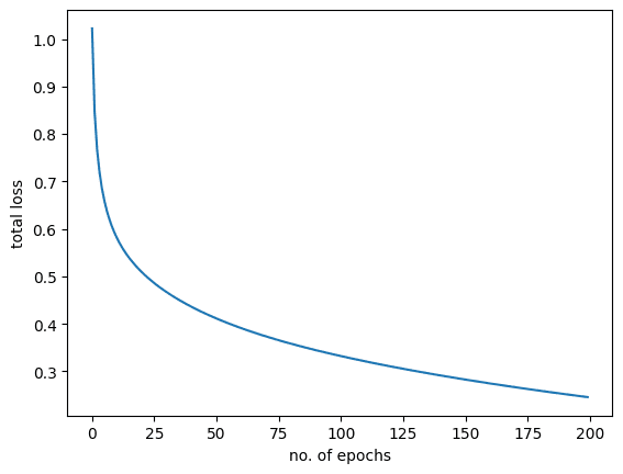
如您所见,模型的精度在每个时期后都会提高,并且其损失会降低。在这里,您使用softmax图像分类器实现的准确率约为85%。如果使用更多数据并增加纪元数,准确性可能会提高很多。现在让我们看看损失和准确性的图是什么样子的。
首先是损失图:
1 2 3 4 | plt.plot(Loss) plt.xlabel("no. of epochs") plt.ylabel("total loss") plt.show() |
应如下所示:
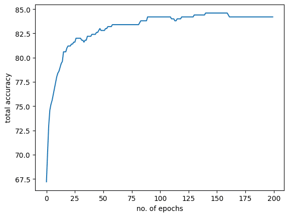
下面是模型精度图:
1 2 3 4 | plt.plot(acc) plt.xlabel("no. of epochs") plt.ylabel("total accuracy") plt.show() |
就像下面的一样:
将所有内容放在一起,以下是完整的代码:
1 2 3 4 5 6 7 8 9 10 11 12 13 14 15 16 17 18 19 20 21 22 23 24 25 26 27 28 29 30 31 32 33 34 35 36 37 38 39 40 41 42 43 44 45 46 47 48 49 50 51 52 53 54 55 56 57 58 59 60 61 62 63 64 65 | import torch import matplotlib.pyplot as plt from torch.utils.data import DataLoader from torchvision import datasets, transforms from torchvision import datasets # download and apply the transform train_data = datasets.FashionMNIST('data', train=True, download=True, transform=transforms.ToTensor()) train_data = list(train_data)[:4000] # splitting the dataset into train and validation sets train_data, val_data = train_data[:3500], train_data[3500:] # build custom softmax module class Softmax(torch.nn.Module): def __init__(self, n_inputs, n_outputs): super(Softmax, self).__init__() self.linear = torch.nn.Linear(n_inputs, n_outputs) def forward(self, x): pred = self.linear(x) return pred # call Softmax Classifier model_softmax = Softmax(784, 10) model_softmax.state_dict() # define loss, optimizier, and dataloader for train and validation sets optimizer = torch.optim.SGD(model_softmax.parameters(), lr = 0.01) criterion = torch.nn.CrossEntropyLoss() batch_size = 16 train_loader = DataLoader(dataset = train_data, batch_size = batch_size) val_loader = DataLoader(dataset = val_data, batch_size = batch_size) epochs = 200 Loss = [] acc = [] for epoch in range(epochs): for i, (images, labels) in enumerate(train_loader): optimizer.zero_grad() outputs = model_softmax(images.view(-1, 28*28)) loss = criterion(outputs, labels) # Loss.append(loss.item()) loss.backward() optimizer.step() Loss.append(loss.item()) correct = 0 for images, labels in val_loader: outputs = model_softmax(images.view(-1, 28*28)) _, predicted = torch.max(outputs.data, 1) correct += (predicted == labels).sum() accuracy = 100 * (correct.item()) / len(val_data) acc.append(accuracy) if epoch % 10 == 0: print('Epoch: {}. Loss: {}. Accuracy: {}'.format(epoch, loss.item(), accuracy)) plt.plot(Loss) plt.xlabel("no. of epochs") plt.ylabel("total loss") plt.show() plt.plot(acc) plt.xlabel("no. of epochs") plt.ylabel("total accuracy") plt.show() |
总结
在本教程中,您学习了如何为图像数据构建 softmax 分类器。特别是,您学到了:
- 关于 Fashion-MNIST 数据集。
- 如何在 PyTorch 中对图像使用 softmax 分类器。
- 如何在 PyTorch 中构建和训练多类图像分类器。
- 如何在模型训练后绘制结果。